
You can have data in BigQuery and a query returning results inside ten minutes. Create a project, create a dataset, upload a CSV, write some SQL. Google documents those clicks better than anyone else is going to, and there is no reason to repeat them here.
What the click-through leaves out is that two of the boxes you tick on the way past are permanent, and two more decide whether the whole thing stays cheap and trustworthy a year from now. Those four are worth an actual conversation.
What BigQuery is, in two sentences
It is serverless — there is no cluster to size, start, or forget to stop. And it is columnar: data is stored column by column rather than row by row, so a query that names two columns reads two columns and leaves the rest of the table on disk.
That second property is the one to hold on to. It explains why BigQuery is fast on very wide tables, and it explains why SELECT * is the most expensive thing you can casually type: it is the one query that guarantees every column gets read.
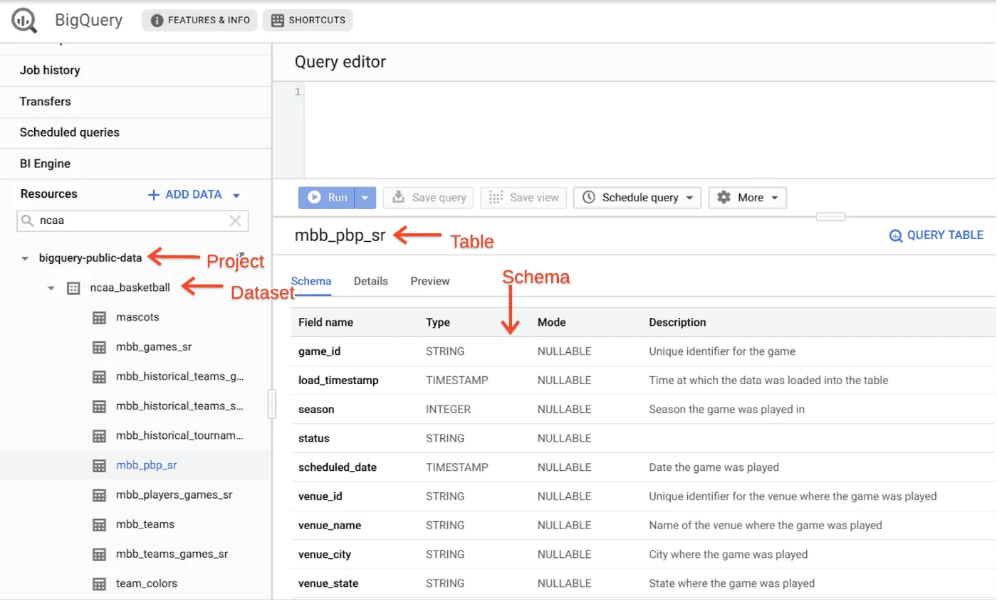
The hierarchy is three levels — project, then dataset, then table. Datasets are where access and location are set, which brings us to the first decision.
Decision 1 — where the dataset lives
When you create a dataset you choose a location, and Google’s documentation is unambiguous about what that choice is worth: “After you create the dataset, the location cannot be changed.” There is no move operation. There is creating a second dataset somewhere else and copying everything into it.
It matters more than a dropdown suggests, because location is also a hard boundary for queries. BigQuery returns an error when the location in a request does not match the location of the datasets in it — and single-region locations do not match multi-region ones, so europe-west4 and the EU multi-region are not interchangeable despite looking like they should be. Two datasets in the wrong two places cannot be joined at all.
Decide the location once, for the whole estate, before the first dataset exists. Take data residency obligations into account while it is still a conversation rather than a migration, and write the answer down somewhere the next person will find it — otherwise they will take the default, and the default is not always the one you picked.
Decision 2 — declare the schema, or let it guess
Auto-detect is a checkbox, and for exploring a file it is the right answer. It is worth knowing exactly what it does, because the documentation describes something narrower than most people assume: “BigQuery selects a random file in the data source and scans up to the first 500 rows of data to use as a representative sample.”
A random file. Up to 500 rows. Everything downstream is inferred from that.
The consequences are ordinary and annoying. A postcode column that happens to be all-numeric in the sample becomes an INTEGER, and the first UK postcode breaks the load. A column that is empty across the whole sample defaults to STRING, whatever it was meant to be. And a CSV whose header row and data rows are all strings will not be recognised as having a header at all — the header arrives as row one of your data, quietly.
The rule that follows is simple: auto-detect while you are exploring, declare the schema the moment a table is something somebody else queries. The point at which a table has a second user is the point at which guessing stops being free.
Decision 3 — the layout, before the data lands
Partitioning and clustering are declared when the table is created, and both work by letting the engine skip data it can prove cannot match — which only happens if queries filter on those columns.
This is why it is a decision rather than a tuning task. It depends on how people will query, not on how the data arrives, and changing your mind later means rewriting the table. Ask which filters will appear in nearly every query — almost always a date, often one entity id — and build for those before the first load.
Decision 4 — the layers
This is the least technical of the four and probably the most valuable. Do not let anything point a dashboard at the table the data landed in.
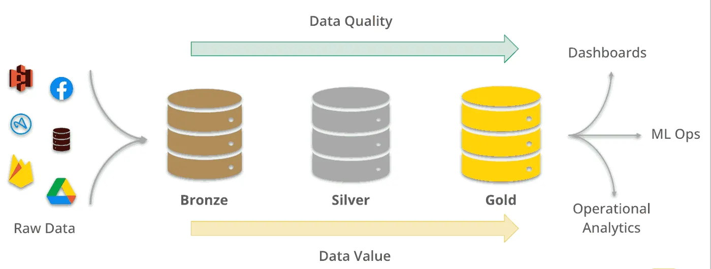
Three layers is enough: raw as it arrived, cleaned and conformed, and a serving layer holding the tables people actually use. Reporting reads the last one only.
The reason is churn. The raw layer gets reloaded, backfilled and reshaped constantly — that is its job — so anything wired directly to it breaks every time someone improves a pipeline. The serving layer changes only when a definition changes, and a definition changing should be a decision somebody made on purpose rather than a side effect of a Tuesday deploy.
This is also why BigQuery sits naturally at the end of an ELT pipeline rather than an ETL one: land the raw data first, then transform it where the compute already is, in layers you can rebuild.
The guardrail to set on day one
BigQuery lets you cap query usage directly. QueryUsagePerDay limits the whole project — it defaults to 200 TiB per day — and QueryUsagePerUserPerDay limits each user and service account separately, which defaults to unlimited.
Set the per-user one. The project ceiling is generous enough that a single person with an unfiltered query on a large table will not come close to it, and that person is the realistic risk, not the department.
Google is refreshingly blunt about the limits of the feature: custom quotas are “approximate”, provide “an additional safeguard against excessive spending”, and are “not designed to strictly limit bytes processed” — BigQuery might occasionally run a query that exceeds one. It is a safety net, not a ceiling. Treat it as the thing that catches an accident, not as a budget.
The takeaway
The console steps take an afternoon and you will not remember them, because you will not need to do them twice. The four decisions take one conversation, and two of them — the location and, in practice, the layout — you get exactly one clean shot at.
Have the conversation before the first CSV.
Originally published on datablast.io in September 2023. Rewritten September 2026.
See it on your own data
20 minutes, your questions, a live walkthrough.